The Capital Assets Pricing Model

Capital Asset Pricing Model

In addition to the Capital Market Line, we will further introduce another important concept: the Capital Asset Pricing Model which is also called CAPM and pronounced “cap M”.

The CAPM is a model that describes the relationship between systematic risk and expected return for assets. The CAPM assumes that the excess return of a stock is determined by the market return and the stock’s relationship with the market’s movement. It is the foundation of the more advanced multi-factor models used by portfolio managers for portfolio construction.

Ok, let’s quickly recap: the systematic risk, or market risk, is undiversifiable risk that’s inherent to the entire market. In contrast, the idiosyncratic risk is the asset-specific risk.

Ok, let’s take a look at CAPM. For a stock, the return of stock i equals the return of the risk free asset plus \beta times the difference between the market return and the risk free return. \beta equals the covariance of stock i and the market divided by the variance of the market.

r_i - r_{f} = \beta \times (r_{m} - r_{f})

r_i = stock return
r_{f} = risk free rate
r_{m} = market return
\beta_i = \frac{cov(r_i,r_{m})}{\sigma^2_{m}}

\beta describes which direction and by how much a stock or portfolio moves relative to the market. For example, if a stock has a \beta of 1, this indicates that if the market’s excess return is 5%, the stock’s excess return would also be 5%. If a stock has a \beta of 1.1, this indicates that if the market’s excess return is 5%, the stock’s excess return would be 1.1 \times 5%, or 5.5%.

Compensating Investors for Risk

Generally speaking, investors need to be compensated in two ways: time value of money and risk. The time value of money is represented by the risk free return. This is the compensation to investors for putting down investments over a period of time. \beta times r_m - r_f represents the risk exposure to the market. It is the additional excess return the investor would require for taking on the given market exposure, \beta . r_m- r_f is the risk premium, and \beta reflects the exposure of an asset to the overall market risk.

When the \beta_i for stock i equals 1, stock i moves up and down with the same magnitude as the market. When \beta_i is greater than 1, stock i moves up and down more than the market. In contrast, when \beta_i is less than 1, stock i moves up and down less than the market.

Let’s look at a simple example. If the risk free return is 2%, \beta_i of stock i equals 1.2 and the market return is 10%. The return of stock i equals 2% + 1.2 \times (10% - 2%) = 11.6.

r_f = 2%
\beta_i = 1.2
r_m = 10%
r_i = 2% + 1.2 \times (10% - 2%) = 11.6%

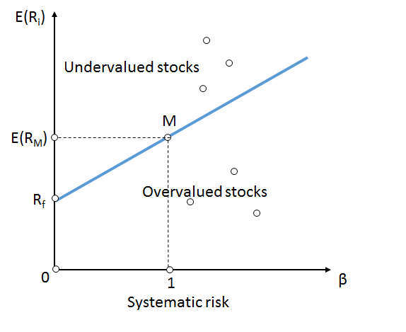
Security Market Line

The Security Market Line is the graphical representation of CAPM and it represents the relation between the risk and return of stocks. Please note that it is different from the capital market line. The y-axis is expected returns but the x-axis is beta. (You may recall that for the capital market line that we learned earlier, the x-axis was standard deviation of a portfolio.) As beta increases, the level of risk increases. Hence, the investors demand higher returns to compensate risk.

The Security Market Line is commonly used to evaluate if a stock should be included in a portfolio. At time points when the stock is above the security market line, it is considered “undervalued” because the stock offers a greater return against its systematic risk. In contrast, when the stock is below the line, it is considered overvalued because the expected return does not overcome the inherent risk.
The SML is also used to compare similar securities with approximately similar returns or similar risks.

This image is from Wikipedia’s page on security market line